Strongly regular Cayley graphs, their representations and eigenvalues

Eigenvalues and characters of Cayley graphs

     When we looked at strongly regular graphs, we noted the powerful results that could be obtained from the eigenvalues of the adjacency matrix.  We found, for example, that the two (16, 6, 2, 2) graphs had eigenvalues 6, 2 and –2, with multiplicities 1, 6 and 9.  In general, strongly regular graphs have just three eigenvalues:  the eigenvalue k equal to the degree of the graph and two other eigenvalues which are roots of the quadratic polynomial

x^2 -(lambda - mu)x - (k-mu).

If the graph is a Cayley graph, with S the neighborhood of the identity,

  

then we may view the graph as existing within the group, in some sense, and we may then use the representations of the group to gain information about this structure.  In particular, if the group is abelian, the characters of the group, when applied to the set S, give the eigenvalues of the graph!

Here are the character values of the abelian group C4 x C4 applied to the generating set S =(x+x^2+x^3)+(y+y^2+y^3).  Notice how in six places the character sends S to 2.  In 9 places, the character values are –2 and in one case (always the trivial representation), the set S is sent to the degree, 6.

A similar picture appears when we look at the Shrikhande graph.  Again the character values give us the eigenvalues! (Here S =(x+x^3)+(xy+x^3y^3)+(y+y^3).)

The fact that character values (on S) are the eigenvalues of the graph is a powerful result.  It comes from the fact that the regular representation of the group decomposes into irreducible representations and the regular representation applied to S is an adjacency matrix of the graph.  The diagonalization of the adjacency matrix parallels to decomposition of the regular representation.

The effect of this result is that we can draw the eigenvalue techniques into the group setting and combine the linear algebra tools with group representation techniques.

The dual Cayley graph

     The characters of an abelian group form a group themselves, under the pointwise product of the functions (fg(x):=f(x)g(x)).  This group, G*, is isomorphic to the original group, G.  Thus we make take a Cayley graph Cay(G,S), fix an eigenvalue theta and create a set S* of the characters which map S to theta.  The dual group G* and the set S* of certain characters gives a Cayley graph Cay(G*,S*).  If the original graph Cay(G,S) is a strongly regular graph then the graph Cay(G*,S*) is also strongly regular.  However, the new graph need not have the same parameters as the original.

However, in all the cases of which I am aware, the dual Cayley graph has the same parameters and is isomorphic to the original.  I think this just shows how few of these I know....  I hope to know more this summer after the NSF-REU at Sam Houston.

More on this later!

Next time: Undergraduate Research Centers in Texas

[Mathematical prerequisites: This article requires an introduction to finite graphs, an elementary introduction to some concepts in matrix theory, and some basic understaninding of group theory]

Follow Ken W. Smith on Twitter @kenwsmith54

Strongly regular Cayley graphs: Introduction

Strongly regular Cayley graphs

Many strongly regular graphs possess high symmetry.  No vertex is different than any other; one may transform vertices in a one-to-one fashion so that the resulting graph is unchanged.   In mathematical terminology, these graphs have automorphisms which act transitively on the vertex set.

The (9,4,1,2) graph is an example of this

 as is the Petersen graph.

The collection of symmetries (automorphisms) of a graph form a group under function composition.  In many cases we may take advantage of this group of symmetries and visualize the vertex set itself as the set of elements of a group.  We do this by picking a "base" vertex to label as the identity element (it does not matter which vertex we choose) and then we label each other vertex in the graph by the group element g which maps the base vertex to the other vertex.

Sometimes this works; sometimes it doesn't.  For example, we can label the vertices of the (9,4,1,2) graph, above, by the elements of the group Z3 x Z3 = {(00),(01),(02), (10),(11),(12), (20),(21),(22)}.  We might choose the red vertex at the top left as the identity, (00), and then agree that its neighbors at the top (green, then blue) be assigned group elements (10), (20), respectively.  The next row (blue, red, green, in that order) are assigned (01), (11), and (21) and the final set at the bottom are (02), (12), (22).  With this assignment, we can think of the vertex (ab) as telling us "move over a and then move down b" in the 3 x 3 square of vertices.

When we can make this construction work, we have a Cayley graph Cay(G,S).  The group G is the group of labels for the vertices and the set S is the neighborhood of the identity element.  The (9,4,1,2) graph is Cay(G,S) where G = Z3 x Z3 and S = {(10),(20),(01),(02)}.

We cannot do this with the Petersen graph.  Although the Petersen graph has many symmetries – there are 120 automorphisms of Petey; they form, Sym(5), the symmetric group on 5 letters – it is not possible to view the Petersen graph as a Cayley graph.  This is because there is no group of order 10 which acts transitively on the vertices of that graph (moving a fixed vertex to any other.)  The cyclic group of order 10 does not act as an automorphism group of the Petersen graph and the dihedral group of order 10, although acting as an automorphism group, is not transitive.  Since there are only two groups of order 10, the cyclic and the dihedral, then we have exhausted our options for a Cayley group in this case.

The Petersen graph is an interesting example; although it cannot be described as a Cayley graph, it can be constructed from 10 cosets of a subgroup of Sym(5).  That subtlety is worth exploring at some point....

A significant research question at this stage is, Which strongly regular graphs are Cayley graphs?  Even if we know a strongly regular graph exists, we are still interested in the question, Does the graph have an automorphism group of size v acting transitively on the points?


A strongly regular Cayley graph is also called a partial difference set (PDS). The terms are almost equivalent; a partial difference set might have the identity 1 in S, in which case our graph has loops.  We forbid loops in our Cayley graphs so a PDS is a (small) generalization of SR Cayley graphs.

The two (16,6,2,2) graphs

In the first blog on strongly regular graphs, we described an SRG with parameters (16,6,2,2), the Shrikhande graph.  There are, in fact, two different (nonisomorphic) SRGs with parameters (16,6,2,2).  Both are Cayley graphs in the group Z4 x Z4. One is the Shrikhande graph; the other is the "rook" graph.  The "rook" graph on n^2 points is obtained by arranging the points in an n x n grid and then assigning adjacency to pairs of vertices that are in the same row or same column.  Thus the reason for the term "rook":  adjacency describes rook moves on the n x n chess board.

The rook graph on the 4x4 board is given below.  In this drawing, each vertex is represented as an element of the group Z4 x Z4.

We may view this graph as a Cayley graph by noting that the neighborhood of the identity (00) is the set of six vertices S={(10),(20),(30),(01),(02),(03)}.

We may represent this group G and set S using multiplicative notation, so that G = C4 x C4 and S = x+x^2+x^3+y+y^2+y^3.  Note that we now treat S as a formal sum, instead of a list.  

In the rook graph, the neighborhood of the identity, 1, has two triangles, drawn in red, below.

On the other hand, the Shrikhande graph is also a Cayley graph.  But here S is different; in multiplicative notation, S is the sum x+x^3+y+y^3+xy+x^3y^3.  When viewed as the neighborhood of the identity, we see, instead of two triangles, a single 6-cycle, (x,xy,y,x^3,x^3y^3,y^3.)  

The difference in the neighborhoods make it clear that these graphs (the rook graph and Shrikhande graph) are truly different; they are nonisomorphic SRGs, even though they have the same parameters.

There are lots of open questions about Strongly regular Cayley graphs.  Many of these are accessible to undergraduates with a course in group theory.  Indeed, this subject will be one of the research topics in the NSF-REU at Sam Houston that I will be directing in June.  Of course, for this reason, there is a lot more I want to say about these interesting objects!  I'll see if I get the time....

Next time: Strongly Regular Cayley Graphs: their representations and eigenvalues

[Mathematical prerequisites: This article requires an introduction to finite graphas and an elementary introduction to some concepts in matrix theory.]

Follow Ken W. Smith on Twitter @kenwsmith54

SRGs II (The linear algebra of strongly regular graphs)

The linear algebra of strongly regular graphs

A graph with vertex set V and edge set E can be encoded in a square array with entries 0s and 1s.  We label the rows and columns of this array by the vertices of the graph and place a 1 in the (i,j) entry if (and only if) the vertex with label i is adjacent to the vertex with label j.  For example, the graph

 has adjacency matrix

Since the adjacency matrix of a graph is a square matrix, then we can consider the linear algebra theory of square matrices and ask questions about eigenvectors, eigenvalues, eigenspaces, minimal and characteristic polynomials and, more generally, pull in many of the powerful tools of linear algebra!

It is natural, at first glance, to ask "Why?"

Why should linear algebra be useful here when all we have done is found a box-like way to encode the graph drawing.  Allen Schwenk, who developed many of the ideas I will cite here, asked that question early in his career.

Just because we find a "box" or "matrix" convenient for collecting the graph data 

-- why should we expect linear algebra to give useful information?? 

This is an example of  "mathematical serendipity" -- it turns out that matrix multiplication encodes the process of "walking" around the graph and so a "geometric" or graph-theoretic concept is simulated by an algebraic one.

Walks on a graph

We need is a simple (but pretty) lemma.

Serendipity Lemma.  If A is the adjacency matrix of a graph then the (i,j) entry in  A^m  is just the number of walks of length m from vertex i to vertex j.

The proof of this lemma will not be given here, but it is straightforward, relying on the definition of matrix multiplication and the fact that the matrix A only has entries zeroes and ones, so that any significant contribution in a product occurs when there is an edge.  If one is comfortable with induction, this is a nice short exercise.

The effect of this lemma is profound.  Powers of the matrix A count walks; the adjacency algebra (linear combinations of powers of A) encode graph theoretic information and so eigenvalues of the matrix (zeroes of the minimal polynomial) carry significant graph theoretic information.  In some cases, the eigenvalues completely describe the graph.

The eigenvalues of a strongly regular graph

In an earlier blog we looked at strongly regular graphs.  A strongly regular graph with parameters (v, k, lambda, mu) has the property that the number of walks of length 2 from a vertex to another takes on one of two values, lambda or mu, depending on whether the vertices are adjacent or not.  This fact gives us an explicit formula for the matrix  A^2.  If vertices i, j are adjacent (so that the (i,j) entry of A is 1) then the (i,j) entry of A^2 is lambda.  If vertices i, j are not adjacent (so that the (i,j) entry of the complementary matrix J-A-I, is 1) then the (i,j) entry of A^2 is mu.  Finally – somewhat trivially – the diagonal entries in  A^2  are all k since there are k walks from a vertex i back to itself.

Thus the matrix A^2 is equal to k times the identity matrix plus lambda times the adjacency matrix plus mu times the complementary matrix J-A-I:

Or, after a bit of rewriting,

This means – here come the most important steps of the linear algebra – that other than the trivial eigenvalue k (with eigenvector equal to a vector of all ones), the other eigenvalues will solve a quadratic equation

(Any eigenvector with eigenvalue not k will be in the nullspace of J and so we may treat the matrix J as zero.)

From this equation, we may find the eigenvalues of the adjacency matrix A.  There are the two roots of this quadratic (often called r and s) and the "trivial" eigenvalue k.

In addition to computing the eigenvalues of the matrix A, we may compute the dimensions of the eigenspaces.  (These are the multiplicities of r and s as roots of the characteristic polynomial of A.)  These dimensions, of course, must be positive integers and that requirement places significant restrictions on the parameters of strongly regular graphs.

With a short bit of programming, one can then generate a list of strongly regular graph parameters and ask, "Does a graph with these parameters exist?"  For the first few graphs on the list, the graph exists and is unique.  As we get deeper into the parameters list, the existence problem gets more difficult and occasionally there are two or more distinct graphs with the same parameters.  But the existence requirements for SRGs seem very restrictive and so it comes as a surprise to discover that the number of SRGs with a certain parameter jumps: there are 3854 different graphs with parameters (35, 16, 6, 8) and eigenvalues 16, 2 and -4!

Next in the list (see the webpage with parameters of SRGs, maintained by Andries Brouwer) is a graph with parameters (36, 10, 4, 2) and eigenvalues 10, 4, –2.  That graph is unique!  There is only one SRG with parameters (36, 10, 4, 2).

Shortly after that. in the list of SRGs, is the parameter set (36, 15, 6, 6) (with eigenvalues 15, 3, -3).  In that case there are (drumroll...) 32548 different SRGs with these parameters!

The eigenvalues 10, 4, -2 uniquely determine the graph while the eigenvalues 15, 3, -3 allow more than 32 thousand graph possibilities.  What a strange world.

Further reading

The Wikipedia article on strongly regular graphs, like many Wikipedia articles on mathematics, is nicely done.
Peter Cameron has a nice article (in pdf) here and a blogpost entry on SRGs and SRGs without triangles.

Anything by Norman Biggs is good; some of those papers are on professor Bigg's website here or on the math arXiv.

Next time: Strongly Regular Cayley Graphs

[Mathematical prerequisites: This article requires an introduction to finite graphas and an elementary introduction to some concepts in matrix theory.]

Follow Ken W. Smith on Twitter @kenwsmith54

The MERiT panel on undergraduate research

Mathematics Education Research in Texas (& undergraduate research)

Recently (Friday, Oct 17, 2014) I had the privilege of being on a panel on undergraduate research, at the MERiT conference in Huntsville, Texas.  Other panelists were Tami Cook, director of the EURECA center at Sam Houston and Kathy Horak Smith, math ed faculty member at Tarleton State University.  The discussion was moderated by Dusty Jones, mathematics educator at Sam.  Each of us, including the moderator, described our experiences with undergraduate research.

Dr. Tami Cook describe her enjoyment of directing undergraduate research in biology and described the development of the undergraduate research center (EURECA) here at Sam Houston.  That center has been open for only a year and Dr. Cook only gets a single course release but she has done a remarkable job in just 12 months, obtaining significant funding for student projects and student travel.  The most significant funding has been for the FAST program (Faculty & student teams) which provides up to $10,000 per summer team (a faculty member and three students) to engage in research or creative endeavors.

I described my experience with undergraduate research, mentioning Ronnie Brown's Carpentry Fable and my summer at the National Security Agency's Director's Summer Program (NSA DSP).  In an attempt to briefly engage my audience (without blackboard or other materials), we iterated some numbers through the 3n+1 problem. I described the Collatz conjecture (hailstone problem) as an example of something easy for undergraduates to understand but (very) hard to solve.  (I will attempt to look at some accessible variations of the Collatz problem in a later post.)

Kathy Horak Smith described her summer work with math seniors in secondary education.  She travels from Tarleton State to Texas Christian University each summer to work with grade school children in an ELL (English Language Learners) math program and takes college students with her.  These college students are engaged in research into mathematical learning, as it is done by young children whose first language is not English.  It was clear from Kathy's exposition that this is an exciting opportunity for her college students and they engage in this professional work with enthusiasm!

Dusty Jones briefly described his summer work with an NSF funded team of five students in the SAM REU.  The students, most of them in an education track, analyzed a variety of grade school statistics textbooks and used the Guidelines for Assessment and Instruction in Statistics Education (GAISE) to evaluate the materials in the textbooks.

Advice from panelists

At the end, we were asked a number of questions about our work.  In response to one question, Tami Cook emphasized the importance of laying out the work expectations for undergrad students at the beginning of a program.  Students needs to be clearly told when work begins, that it will be full-time. The ground rules for work should be laid out early.  Yes, there is much flexibility within any research program (NO, we don't have to start at 8!) but many undergraduates do not really understand either full-time work nor what it means to work 40 hours a week on a science project.  Don't soft-pedal the work involved; the really good students are eager to work hard and dive into the research!

In response to another question, Kathy emphasized the importance of high, professional expectations for our students. If we describe professional expectations, many of our students are eager to step up to those expectations!  They will make mistakes, of course, but the value of the undergraduate research program is to introduce students to their profession.  They are eager to become professionals and are ready to quit being students!  Respect that desire!  (Yes, in my experience directing math research, I can ask my students to learn LaTeX, install GAP or Sage, and although some faculty think that we should not expect this of undergrads, by the time I turn around, the students are done and eager to move on to the next task.)

The presentations were well received by conference participants, with a number of questions after the formal end of the panel and during the lunch that followed.  It was an enjoyable experience to discuss undergraduate research in this setting.

Next time: The linear algebra of strongly regular graphs

[Mathematical prerequisites: This article requires no mathematical background.]

Follow Ken W. Smith on Twitter @kenwsmith54

Strongly regular graphs, I

Strongly regular graphs

Strongly regular graphs "stand on the cusp between the random and the highly structured", says combinatorialist Peter Cameron.  The conditions for the existence and the construction of strongly regular graphs provides a rich source of mathematical investigation, with many applications to algebra, linear algebra and combinatorics.

A graph is regular if every vertex has the same degree.  Let's use the letter k for the degree of our regular graph.

A regular graph is strongly regular if the number of walks of length 2 between two different vertices depends only on the adjacency of the two vertices.  We let  lambda  count the number of paths of length 2 between adjacent vertices and set  mu  as the number of paths of length 2 between non-adjacent vertices.

Given adjacent vertices x and y (in the figure below), the parameter  lambda  counts the number of vertices z adjacent to both.

But if x and y are not adjacent (below), mu counts the number of vertices z in this second configuration.

The parameters of a k-regular graph on v vertices are written as a 4-tuple (v, k, lambda, mu).  The graph below, on 9 vertices, with degree 4, is an example of a (9, 4, 1, 2) strongly regular graph (SRG.)  Each edge (adjacent pair) is on exactly 1 triangle, but each nonadjacent pair form the opposite corners of a 4-cycle and so there are mu=2 walks of length two between the nonadjacent vertices.

The Petersen graph, below, is an example of a (10, 3, 0, 1) SRG.

It is possible for mu and lambda to be equal.  Here (below) is the Shrikhande graph, an SRG with parameters (16, 6, 2, 2).  (This graph was found by S. S. Shrikhande.  I was privileged to work for some time at Central Michigan University with Mohan Shrikhande, son of S. S. Shrikhande.  Both father and son live in Mt. Pleasant, Michigan.)

There is (of course) a nice Wikipedia article on SRGs.  The drawing, above, have been copied from that article.

Fundamental existence question & conditions

A fundamental question in the study of strongly regular graphs is simply, "For which parameters (v, k,  lambda, mu) does there exist a SRG?"  The current progress on this question can be summarized in the tables kept by Andries Brouwer in Eindhoven, Netherlands.  

One first step to eliminating false parameter sets is the "First feasibility condition" created by counting ordered pairs of vertices (y, z) in the configuration below.

We fix the vertex x and count vertices y, z where x and y are adjacent, as are y and z, but x is not adjacent to z.  Given x, there are k choices for the vertex y and then k-lambda-1 choices for z.  (There are k vertices adjacent to y but one of those is x and there are another lambda which are adjacent to x.  Throw those out....)  So, given x, there are k(k-lambda-1) configurations like that, above.

On the other hand, given x, we can hunt for vertices z first -- there are v-k-1 choices for z -- and then hunt for y -- there are mu choices for y once we find z and so there are (v-k-1)mu  configurations like that, above.

Since we got two results for the same count, we know they must be equal and so we have the following condition on the parameters (v, k, lambda, mu) of a SRG:

k(k-lambda-1) = (v-k-1)mu

This is the "first feasibility condition" for SRGs.  There are a few more feasibility conditions, involving more subtle arguments.  We will explore two of those in a later post.

Open parameter sets

Meanwhile, just so one realizes that there are LOTS of open questions on strongly regular graphs, we mention a few "existence" questions here.  It would be very nice to either construct or rule out SRGs with the following parameters:

(65, 32, 15, 16)

(69, 20, 7, 5)

(75, 32, 10, 16)

...

(96, 35 10, 14)

(96, 45, 24, 18)

(99, 14, 1, 2)

(100, 33, 8, 12)

...

(120, 35, 10, 10)

...

(144, 52, 16, 20)

...

(160, 54, 18, 18)

(162, 21, 0, 3)

...

Of the many open cases, I have pulled out in the list above, the parameters that I (and others) find most interesting.  Most of these cases are quite hard and the discovery of a single graph in the list above would be a publishable paper!  (Write me!  Did I mention my Erdos number is 2?!)

All strongly regular graphs on 64 or fewer vertices have been found by exhaustive computer search by Ted Spence.  One might note that there are exactly 32548 distinct (nonisomorphic) graphs with parameters (36,15,6,6).

I have worked pretty hard on the parameter set (99,14,1,2).  A doctoral dissertation in computer science by Majid Behbahani (2009, here in pdf) attempts the most obvious constructions for this strongly regular graph and does not find it.  This does not rule out this SRG but makes it clear that a construction will be somewhat unusual.  In the same vein, Makhnev and Nosov describe a search for the graph (162,21,0,3).   I've also looked into (120,35,10,10) and (160,54,18,18); in both cases there is no abelian Cayley graph with these parameters.  (More on that later.)  

A strongly regular graph with parameters (3250,57,0,1) is an example of a Moore graph.  Many of us in algebraic combinatorics have looked for that graph and it still eludes us.

It turns out that the most powerful tools for the study of strongly regular come from linear algebra.  That will be the subject of the next post.

Next time: The MERiT conference & undergraduate research.

[Mathematical prerequisites: This article requires a basic introduction to graph theory.]

Follow Ken W. Smith on Twitter @kenwsmith54

COURI and EURECA, promoting undergraduate research across campuses

COURI

Last Thursday, while visiting professor Art Duval at the University of Texas at El Paso (UTEP), I had the privilege of spending about an hour with Lourdes Echegoyen, UTEP's director of the center for undergraduate research.  The UTEP center, now called COURI (Campus Office of Undergraduate Research Initiatives) has a full time director (Dr. Echegoyen is a member of the Chemistry faculty), full-time staff, and is even now advertising for an associate director!

The COURI center has expanded interest across campus in undergraduate research.  One way undergraduate research is promoted is through a campus-wide zero-credit class that interested students may take prior to pursuing undergraduate research.

The Center and faculty are active in promoting undergraduate research in every discipline but much research interest comes from science faculty.  The faculty and staff involved in COURI have received several federal grants and are encouraging the development of NSF-REU proposals, although most of their emphasis seems to be on year long, in-house programs.  (In the long run, year long, in-house programs are much more beneficial to students than short summer programs.)  The UTEP on-campus programs have even begun receiving applicants from China as Chinese colleges offer to fund student travel and pay UTEP tuition.  The UTEP undergrad research programs have also recently begun engaging in an exchange program with universities in Mexico.

Dr. Echegoyen is a very energetic individual.  I suspect she spends 60 hours a week administrating, organizing, promoting undergraduate research at UTEP.  It was fun to talk to her about undergraduate research!

During our conversation, I wondered out loud about the possibility of exchanging students in some way, maybe recruiting Sam Houston students to UTEP, or vice-versa, to engage in undergraduate research.  Could we set up some type of online math connection between people at our two schools?

EURECA

Sam Houston State University also has a center for the promotion of undergraduate research.  Although only a year old, the center, Enhancing Undergraduate Research and Creative Activities (EURECA), has a director, Dr. Tami Cook (Biology faculty), two graduate assistants, a budget, and is actively promoting undergraduate research across our campus.  Last summer eight student research teams were funded by EURECA, with the aid of college deans.  These Faculty and Student Team (FAST) summer awards pay both students and faculty.  A faculty member leads a team of typically three students, working on a research project for ten weeks of the summer.  The faculty member is paid $4000 and the students are paid $2000.  Although these stipends are about half of the NSF-REU stipends, they are a good start towards promoting undergraduate research!

Students involved in the FAST summer programs at Sam Houston State University often continue to engage in research with their professor after the formal summer project ends.  (Some had already begun research before the summer funding stimulus.)  In the spring following the summer project, the students present their work on campus at the annual Undergraduate Research Symposium sponsored by the Honors College at Sam Houston.

If I may boast for a moment (this is my blog!) -- I chaired the committee that developed EURECA center and so, of course, I am very proud of that program.  Please read more about the recent developments here!

Next time: Strongly regular graphs

[Mathematical prerequisites: This article requires no mathematical background.]

Follow Ken W. Smith on Twitter @kenwsmith54

Feeding a Family of Four

A statistics student, some time back, posted on Facebook a joke about (1) a large pizza, (2) statisticians, (3) applied mathematicians and (4) theoretical mathematicians.  The punch line was that the first three could each "feed a family of four." 

At the time, the joke seemed to be aimed at “the other half” of our department program, at our students in theoretical (pure) mathematics. As  graduate coordinator in our pure math program, I took the post a little personally.  My frustration with the joke was not just that it seemed to say, “We [stat students] are better than you — we will get jobs and you won’t!” but that it was simply wrong.  

There seems to be a strong demand for students in a theoretical (or “pure”) math program, but a popular belief in our cultural is that all mathematicians ever do is teach.  

Why hire theoretical mathematicians?

A mathematician learns to solve a vague, fuzzy problem by organizing the problem into a coherent form and then using various tools to attack this coherent problem.  Since every problem begins with a vague, poorly defined stage, these problem-solving tools are valuable in industry and in applied mathematics, even if the original training is theoretical.  

Higher education often trains people to be specialists, to be excellent in a narrow field. This can be very good.  We need chemical engineers, actuaries, statisticians, mathematical biologists, petroleum engineers … and nurses and doctors.  But training in theoretical mathematics tends to avoid this specialization, concentrating instead of deep understand of general mathematical principles.  This creates a certain tension in the job market — do companies prefer a specialist, assigned to a particular task, or a generalist who is good at solving problems of all types?  It depends….

From my experience, both specialists and generalists have their place, but it is foolish to require education to focus on a single small specialty.

An undergraduate student timidly knocked on my office door one afternoon, several years ago.  I invited her in and she began to discuss her “problem.”  She liked math but didn’t want to teach.  Her dad wanted her to be a chemist because he wanted her to have a real job (like he did.)  He was convinced that if she pursued her desire to major in math then she would have to be a teacher if she wanted to have a paycheck.  After we chatted a bit, I wrote her a long email (meant to be read by dad) that laid out all the various job opportunities available in mathematics.  Eventually she majored in math, did an undergraduate research project in statistics (yes, statistics!) and received a large fellowship to pursue doctoral studies at a major university.  Yes, you can love mathematics and get paid a lot of money.  (And no, you won’t be teaching.  Obviously if you are making a lot of money, you are not teaching....)

One of our graduate students had a similar problem.  Her father worked for a major international corporation which builds agricultural machinery.  He wasn’t very eager for his daughter to get a masters degree in mathematics because he wanted her to get a job after school.  The delightful part of this story is that after her masters degree, a certain company interviewed her and, due to her mathematical training, offered her a job with a salary higher than her father’s.  What company was interested in her mathematical training? The same company that her dad worked for!   (It was just a different branch.)

Around 1990, I spent a year at the National Security Agency (NSA) as part of a mathematical sabbatical.  The National Security Agency has literally thousands of mathematicians working there (probably over ten thousand -- but the exact number is classified.)  Outside the NSA there are more thousands of mathematicians working for the various defense contractors such as Westinghouse.  (There are also defense contractors in other parts of the country, including Texas.)

Our cell phone technology would not exist without the mathematicians who design the codes to carry the digital signals.  Our internet commerce would not exist were it not for the mathematicians who designed the public key encryption schemes that allow us to securely exchange information through computer servers.

How is this related to undergraduate research?

Underneath the belief that "all you can do with math is teach it", is a belief that mathematics is a dead subject.  Vibrant, growing fields require that people engage in that field; dead, stagnant subjects only have room for teachers.

There are a variety of ways to emphasize the explorative processes in the growing field of mathematics.  Certainly one of the best ways to communicate the living nature of mathematics is to get students engaged in research in the subject!

Some resources

Here I've tried to collect some online sources that talk about the importance of mathematics and its value is science and society.


A recent NPR article describes the search for mathematicians to analyze big data.

A Wall Street Journal article describes the career of mathematician as one of the top, most desired jobs.

One of my favorite blogs to read is FutilityCloset; the blog has an interesting story, "Augury", on the connections between math and science.

Stanford mathematician, Keith Devlin, teaches a MOOC on mathematical thinking.

The Mathematical Association of America has some webpages devoted to the question, "What can I do with a math major?"  Here are some of the sample careers off of the MAA web page:

http://www.maa.org/careers/denbleyker.html  (Janet denBleyker -- actuary)

http://www.maa.org/careers/sford.html 

http://www.maa.org/careers/monticino.html

http://www.maa.org/careers/murray.html (Math major whose interests led him into computer science)

http://www.maa.org/careers/lentz.html  (Biostaticians whose interests led her on to a Ph.D. in animal science)

http://www.maa.org/careers/stabbe.html (Math major whose mathematical training eventually lead him to law school.)

Mathematicians are sought after in almost every area of industry.  The US government has been trying to fix the "crisis" in math and science for some time.  Earlier in this decade (about 2005) Congress had a committee look into the decline in American capabilities in science and technology.  The result was a report, "Rising Above the Gathering Storm: Energizing and Employing America For A Brighter Economic Future."  That report suggested some significant changes in the way the US prepares people for industry.  The top suggestion, coming from that investigation, addressing the country's greatest need, was:  "Action A-1: Annually recruit 10,000 science and mathematics teachers by awarding 4-year scholarships and thereby educating 10 million minds."

The reason for making STEM teaching a top priority is simply that we don't have enough people trained in science and math for the country's needs.  And to get good mathematicians, we need more math teachers!  Now, a lot of people have focused on the "teaching" part of this statement, but the reason the report mentions teachers is because the country desperately needs their students!  There are NOT enough math majors in this country for the jobs we have!

Next time: COURI & EURECA, promoting undergraduate research across campuses.

[Mathematical prerequisites: This article requires no mathematical background.]

Follow Ken W. Smith on Twitter @kenwsmith54

Randomly decomposable graphs, III (open questions in RDGs)

Some open questions in RDGs

In this third post on randomly decomposable graphs, we explore some open questions accessible to undergraduate students.  Partial results on these questions, for selected graphs, have just begun to appear in the mathematical literature and there are many, many trails to be explored in this area of the mathematical wilderness!

Fix a graph H and explore the poset RD(H) of all graphs G which are randomly decomposable with respect to H.  Recall that the height of a graph G in this poset is the number of edge-disjoint copies of H required to make G.  If the height of G is the integer a  and if H has q edges then G has e=aq edges.  A graph G is abundant with respect to H if there are more than a copies of H in G; G is trivial with respect to H if there are exactly a copies of H in G.  Thus the poset RD(H) partitions into two sets, the set,  RD_0(H), of trivial randomly decomposable graphs, and the set RD_A(H) of abundant randomly decomposable graphs.  Since H itself is a trivial member of RD(H), we can ask for minimal members of RD_A(H), that is, graphs which are abundantly RDG but have no subgraphs which are.

With this brief review, some basic mathematical questions jump out at us.

1. Given a fixed graph H, classify completely the members of RD(H).
2. Given a fixed graph H, list the minimally abundant members of RD(H).
3. Classify graphs H for which there are no abundant RDGs, that is, for which RD(H)=RD_0(H).
4. Are there graphs H for which RD(H) is finite?  Indeed, is it possible that RD(H)={H} for some graphs?

The first two questions invite experimentation with small graphs.  Choose a graph H with just 3 or 4 edges and first attempt to find the smallest abundant members of RD(H).  A helpful result in this area is the following lemma: 

"If G is minimally abundant with respect to H then the height of G 

is bounded above by the number of edges of H."  

Thus if H has only three edges, one need use at most three copies of H in building these smallest abundant RDGs.

If it is relatively easy to describe the minimal elements in RD_A(H), maybe it is possible to describe all of RD(H).  This has been done for graphs with two edges, and for the graphs H=P_3 and H=K_3 with three edges.  It has also been done for a few small paths and should be done for graphs with three or four edges.  Although describing RD(H) is somewhat easy for a few graphs (like H=K_3) this gets surprisingly difficult for other graphs (like H=C_4.)

Some graphs cannot create abundant RDGs.  This is true for the complete graphs, H=K_n, in which there are too many edges to allow one to build up RDGs that have "extra" copies of H.  Are there other graphs with this property?  Surely there are ... so can we classify, in some way, those graphs for which every RDG is trivial?

If H is connected then the graph aH, consisting of a components, each isomorphic to H, is in RD(H) and so the poset RD_0(H) is infinite.  But if H is not connected, then maybe RD(H) could be finite? When is RD(H) finite?  

I can argue that if H is the graph with three edges on five vertices, below,  formed from the path of length two and a disconnected edge, then RD(H)={H}!  (That graph, H = P_2 + K_1, is drawn below, using output from the Sage software program.)

For the student just beginning to explore RDGs: take a notebook and pen (or pencil) and draw a small graph H with three or four edges.  You might wish to choose one of the graphs drawn below.

Then begin constructing members of RD(H).  See if you can develop the first few members of RD(H) that involve 2, 3 or 4 copies of H.  Can you detect a pattern?  Can you make a statement about trivial or abundant graphs?  Drop me a line at kenwsmith54 (at) gmail (dot) com!

[Mathematical prerequisites: This article requires a basic introduction to randomly decomposable graphs (as seen in the previous  few blog posts).]

Follow Ken W. Smith on Twitter @kenwsmith54

Randomly decomposable graphs, II (concentrating on paths)

Abundant vs. trivial decompositions of a graph

In the previous post, we introduced randomly decomposable graphs, looking for the set, RD(H), of all graphs randomly decomposable with respect to a fixed graph H.

For example, if H is the path P_3, with four vertices and three edges, then there are five graphs, each with six edges which are in RD(H).  These five graphs include one disconnected graph, the graph which is two disconnected copies of P_3.  The four connected graphs are drawn below, with two edge-disjoint paths of length three drawn in different colors, one path in blue and another in red.  In each case, the removal of any path of length 3 leaves a path of length 3.

Note that although each of the graphs drawn above is clearly decomposable into two copies of P_3 (as indicated by the two colors, blue and red), there are LOTS more copies of P_3 in these graphs.  Indeed, the graph, C_6, on the left, has six copies of P_3, while the "bowtie" (second from the left) has (I think) eight copies of P_3, the complete graph K_4, third from left has six paths of length 3 and the rightmost graph (K_{2,3}) has 12.

Since there are so many copies of H in these graphs, it is not easy to show that these graphs are randomly decomposable.  On the other hand, if a graph G is constructed from  a  edge-disjoint copies of H and there are only  a  copies of H in G then the decomposition of G into copies of H is trivial.  For example, let us change H and set H to be the triangle (3-cycle) K_3, with 3 vertices and 3 edges.  Then the "bowtie" graph, above (second from the left), is trivially decomposable into copies of K_3 since it is the edge-disjoint union of  a=2 copies of K_3 and there are only two copies of K_3 in the graph.

If H has q edges and a graph G with e=qa edges decomposes into  a  edge-disjoint copies of H then we say G is trivially randomly decomposable with respect to H if there are only a copies of H in G.  If, instead, G has more than  a  copies of H, then we say that H is abundant in G.

The four graphs in the figure at the top of this blog all have H=P_3 as an "abundant" subgraph since  a=2 but there are, in each case, more than two copies of P_3.  On the other hand, if H=K_3, the bowtie graph is trivially decomposable since the two copies of K_3 used to construct the bowtie are the only copies of K_3 in the graph.

We make the distinction between trivial decompositions and abundant decompositions simply because we are not really interested in trivial decompositions.  We want an interesting problem.  The randomly decomposable graphs which are trivially decomposable are not interesting but the abundant graphs are.

The poset of randomly decomposable graphs and its trivial/abundant pieces

The set of finite graphs form a partially ordered set ("poset") ordered by the concept of subgraph. So the set RD(H) will also be a poset, with one member, G1, being less than another, G2, if G1 is a subgraph of G2.  It should be clear that this poset can be arranged by the height  a; at the bottom of the poset is H, immediately above H are the graphs which can be constructed from two copies of H; above those are the graphs constructed from three copies of H and so on.

If G1 is below G2 in the poset of randomly decomposable graphs (RDGs), then if G2 is trivially decomposable, so is G1.  The concept of "trivially" randomly decomposable is preserved by going down in the poset and so it is natural to ask if there are any maximally trivial RDGs.  These would be graphs which are trivially randomly decomposable but no graph above them is.

In a similar way, the concept of "abundantly" decomposable is preserved by going up the poset of RDGs, adding copies of H to graphs on a lower level.  If G1 is below G2 in the poset of RDGs, then if G1 is "abundant", so is G2.  Now H is trivial, not abundant, so given an abundant graph, we can always work ourselves down the poset of RDGs, removing a copy of H each time, until we reach a minimally abundant RDG, one which has no abundant subgraphs.  Thus minimally abundant RDGs sit at the cusp of "trivial" (uninteresting) RDGs and "abundant" (and complicated) RDGs.

Paths

We might begin our study of RDGs by beginning with the simplest graphs, the paths.  If P_n is a path of length n (and so has n+1 vertices and n edges) then what does RD(P_n) look like?  Since P_n is a connected graph, then if G is in RD(P_n), each connected component of G is also in RD(P_n) and so we can just concentrate on the connected members of RD(P_n).  There are only five connected members of RD(P_3).  They are:

The set RD(P_3) is then just a union of a finite number of copies of graphs from the set above. The four graphs on the left are of height 2; the rightmost graph is just H=P_3.  The poset RD(P_3) is infinite; a graph in that set is "abundant" if at least one of its components is from the first four graphs drawn on the left.  (Stated another way, a graph in RD(P_3) is "trivial" only if it is a disconnected union of copies of P_3.)

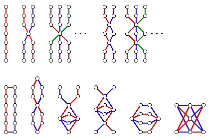
Below, off the webpage of Robert Molina (Alma College), in collaboration with Myles McNally (also at Alma) is a summary of all connected members of RD(P_4):

Since the number of edges in P_4 is even, there is an infinite set of connected graphs in which the paths are all joined in the middle.  This infinite set is represented by the three dots.

Here, from work of McNally & Molina, are the connected members of RD(P_5).  Note that this set is finite.  The first three graphs are predictable (to me) but the last two are rather strange. 

And here the connected members of RD(P_6).  Since the number of edges is even, we have some infinite families

but then a few more strange objects towards the end.

If H=P_7 then we have one infinite family (involving paths pinched at two points); we have the cycle and a figure eight ... and then ten more strange objects that would be hard to find without a computer.

H=P_8 is more of the same:

By the time our paths have 9 edges, the members of RD(P_9) are too many to draw here.  A few are given below.

All the members of RD(P_9) are available on the webpages maintained by McNally & Molina.  Picture of RD(P_9), RD(P_10) can be found at http://othello.alma.edu/~molina/rd(pk).html.  These graphs include collections of objects McNally & Molina call "braids", "twisted braids" and "branch growths."

And we have only begun looking at paths!!  What if H is more complicated?!

The Two-Path Conjecture

Along the way, as a number of us looked at RD(H) where H was a path, we began to believe that anytime we connected two copies of the path P_n, there were always additional copies of P_n created in that process.  No connected member of RD(P_n) of height two was trivial.  This eventually became a conjecture: 

The two-path conjecture.  Let G be the connected edge-disjoint union of two paths of length n. Then there are more than two copies of P_n in G.

With the help of Doug West and Herb Fleischner, we were able to prove that conjecture and publish the result.  (That paper is available here or here.)

and Erdos numbers

Many mathematicians encourage collaboration by keeping track of the "collaboration graph", in which two mathematicians are joined by an edge if they have collaborated on a published paper.  By tradition, the center of this collaboration graph is Paul Erdos.  It so happens that Doug West has Erdős number 1 so any other author of the paper on the Two-Path Conjecture has Erdos number 2. So I have Erdos number 2. (As it happens, I had earlier co-authored a paper with Allen Schwenk, who wrote a paper with Erdos, so I already had Erdos number 2.)

So ... if your Erdos number is higher than 3 (or does not yet exist!) you can get an Erdos number of 3 by publishing with me!  ;-)  Pick one of our open problems on one of these blogs, play with it a bit and write me an email.  Let's take a hike together in the mathematical wilderness!

Next time: RDGs, Part 3, some open questions in randomly decomposable graphs

[Mathematical prerequisites: This article requires a basic introduction to graph theory (as seen in the previous blog post).]

Follow Ken W. Smith on Twitter @kenwsmith54